We use cookies for analytics and advertising. Ads are disabled until you accept advertising cookies. Read our Cookie Policy and Privacy Policy.
Partitioning & Sharding Strategy for Ultra-Large Datasets | TVerge Tech
Partitioning & Sharding Strategy for Ultra-Large Datasets
A deep dive into declarative range and hash partitioning in PostgreSQL and MySQL, plus when to move from partitioning to sharding with Citus for ultra-large tables.
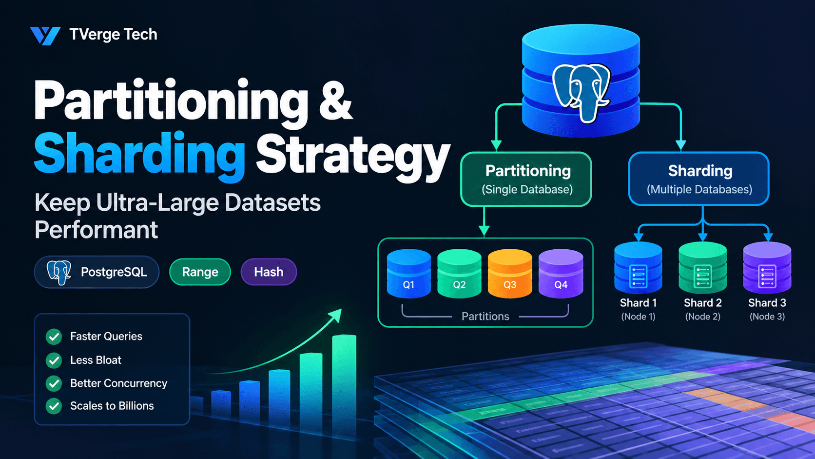
Partitioning & Sharding Strategy: Implementing Declarative Table Partitioning by Range or Hash to Keep Ultra-Large Datasets Performant
When a table crosses hundreds of millions of rows, the symptoms show up everywhere at once: VACUUM runs for hours, index bloat creeps into gigabytes of dead weight, a single DELETE locks up the application, and a query that used to return in 40ms now takes four seconds because the planner is scanning a heap it can no longer hold in memory. This is the point where "add another index" stops working and the real fix — dividing the table itself — becomes unavoidable.
This guide walks through the two techniques that solve this at different layers of the stack: declarative partitioning, which splits one logical table into smaller physical tables inside a single database instance, and sharding, which splits data across multiple database instances or nodes entirely. We'll cover range and hash partitioning in depth, show working DDL, and explain when partitioning alone is enough versus when you actually need to shard.
Partitioning vs. Sharding: Two Different Problems
It's easy to use these terms interchangeably, but they solve different bottlenecks.
Partitioning happens inside a single database engine. The table orders might look like one table to every query and every application, but under the hood it's actually a parent "routing" object with no rows of its own, pointing to a set of child tables (partitions) that each hold a slice of the data. The engine — PostgreSQL, MySQL, or otherwise — handles routing inserts to the right partition and pruning irrelevant partitions out of a query plan automatically. Your compute and storage are still on one machine (or one primary plus replicas); you're just organizing the data more intelligently.
Sharding happens across machines. Data is split by some key (a tenant ID, a customer ID, a geographic region) and each shard lives on its own database node with its own CPU, memory, and disk. Sharding solves the problem partitioning cannot: when a single machine's compute or storage ceiling is the actual constraint, not just query planning inefficiency.
A useful rule of thumb: reach for partitioning first. It's native, well-supported, and solves the majority of "table too large" problems without adding distributed-systems complexity. Reach for sharding only when partitioning has been exhausted and a single node genuinely can't hold the working set or the write throughput you need.
Why Partition at All? The Concrete Benefits
Partition pruning — the query planner eliminates entire partitions before touching them at all, based on the WHERE clause. A query filtering on a date range only has to scan the one or two monthly partitions that could possibly match, not the whole table.
Cheaper bulk operations — dropping a partition to purge old data is a metadata operation. Compare that to running DELETE FROM orders WHERE created_at < '2023-01-01', which has to visit every matching row, generate WAL for every one, and leave a pile of dead tuples for VACUUM to clean up afterward.
Smaller, more effective indexes — each partition gets its own index, so a lookup only has to walk an index sized to that partition, not the entire dataset. Hot partitions are more likely to stay resident in memory.
Tiered storage — older, cold partitions can be moved to slower, cheaper storage while active partitions stay on fast disks.
Maintenance isolation — a VACUUM, REINDEX, or ANALYZE on one partition doesn't have to lock or scan the entire table.
Declarative Partitioning in PostgreSQL
PostgreSQL has supported native declarative partitioning since version 10, and it's the only approach worth using for a new schema today — the old pattern of table inheritance plus triggers is a legacy workaround that predates the PARTITION BY syntax and is harder to maintain correctly. The official reference is the PostgreSQL documentation on Table Partitioning.
PostgreSQL supports three declarative strategies: Range, List, and Hash. This article focuses on Range and Hash, since those are the two used to keep ultra-large, high-velocity tables performant.
Range Partitioning
Range partitioning divides rows by an ordered key — almost always a timestamp or a sequential ID — into non-overlapping bands. It's the natural fit for time-series data: events, logs, orders, metrics, anything that's naturally append-only and queried by recency.
-- Parent table: defines the shape, holds no rows of its own
CREATE TABLE events (
    id          bigint GENERATED ALWAYS AS IDENTITY,
    created_at  timestamptz NOT NULL,
    event_type  text NOT NULL,
    payload     jsonb,
    PRIMARY KEY (id, created_at)
) PARTITION BY RANGE (created_at);

-- Monthly partitions
CREATE TABLE events_2026_08 PARTITION OF events
    FOR VALUES FROM ('2026-08-01') TO ('2026-09-01');

CREATE TABLE events_2026_09 PARTITION OF events
    FOR VALUES FROM ('2026-09-01') TO ('2026-10-01');

CREATE TABLE events_2026_10 PARTITION OF events
    FOR VALUES FROM ('2026-10-01') TO ('2026-11-01');
A detail worth memorizing because it trips up almost everyone the first time: the lower bound in FROM is inclusive, and the upper bound in TO is exclusive. In the example above, a row with created_at = '2026-09-01 00:00:00' belongs to the September partition, not August — this is what lets adjacent ranges meet cleanly with no gap and no overlap.
Because the primary key on a partitioned table must include every column used in the partition key, PRIMARY KEY (id, created_at) is required here, not just PRIMARY KEY (id). This is one of the most common migration blockers: an existing single-column primary key or unique constraint has to be widened to include the partition key before the table can be converted.
Once a range-partitioned table is in place, a query like:
SELECT count(*) FROM events
WHERE created_at >= '2026-09-15' AND created_at < '2026-09-20';
only touches events_2026_09 — every other partition is pruned at plan time. You can confirm this yourself with EXPLAIN (ANALYZE, BUFFERS); the plan will show a Partitions removed count under the Append node, confirming the untouched partitions were never scanned.
Hash Partitioning
Hash partitioning is the right tool when there's no natural range to partition by, but you still need to break a huge table into more manageable, evenly-sized chunks — for example, partitioning a users or accounts table by ID purely to shrink index and vacuum overhead, with no time-based or categorical structure to lean on.
CREATE TABLE accounts (
    id          bigint NOT NULL,
    org_id      bigint NOT NULL,
    email       text NOT NULL,
    created_at  timestamptz NOT NULL DEFAULT now(),
    PRIMARY KEY (id)
) PARTITION BY HASH (id);

CREATE TABLE accounts_p0 PARTITION OF accounts
    FOR VALUES WITH (MODULUS 8, REMAINDER 0);

CREATE TABLE accounts_p1 PARTITION OF accounts
    FOR VALUES WITH (MODULUS 8, REMAINDER 1);

-- ... repeat through REMAINDER 7
Each partition owns one "bucket" out of the modulus, and Postgres routes each row into a bucket based on a hash of the partition key. This distributes rows roughly evenly regardless of the actual values, which is exactly the point: there's no meaningful ordering in an account ID, so there's nothing to range-partition on, but the table still benefits from being split into eight (or sixteen, or thirty-two) smaller physical tables instead of one enormous one.
The tradeoff versus range partitioning is that hash partitions can't be pruned as effectively for range-style queries (WHERE id > 1000), and you can't simply drop an old hash partition the way you can drop last year's range partition — the data isn't organized by age or category, so every bucket keeps growing indefinitely. Pick your modulus with future growth in mind, since increasing the number of hash partitions later means rehashing and physically moving data.
List Partitioning, Briefly
The third declarative method, list partitioning, splits rows by an explicit set of discrete values — for example, partitioning a table by region_code IN ('us-east', 'us-west', 'eu-west'). It's less commonly the answer for "ultra-large dataset" problems specifically, but it's worth knowing it exists for categorical data with a small, known set of values, and it's documented in the same PostgreSQL reference above.
Partition Pruning and the Planner
Partition pruning is controlled by the enable_partition_pruning setting, which defaults to on, and it happens both at plan time (when the filter values are known at parse time) and at execution time (when the filter arrives as a bind parameter, e.g. from a prepared statement). This is why writing your WHERE clause to directly reference the partition key — rather than wrapping it in a function or an implicit cast — matters: pruning can only eliminate a partition if the planner can prove, from the clause as written, that the partition's bound range cannot satisfy it.
A common mistake: filtering on DATE(created_at) = '2026-09-01' instead of created_at >= '2026-09-01' AND created_at < '2026-09-02'. Wrapping the partition key in a function often defeats pruning entirely, because the planner can no longer directly compare the column's raw value against each partition's bound.
MySQL's Partitioning Model
MySQL has supported user-defined partitioning since 5.1, currently documented in Chapter 26, "Partitioning" of the MySQL 8.0 Reference Manual, and it supports the equivalent RANGE, LIST, HASH, and KEY methods, plus subpartitioning (composite partitioning) for a second level of division within each partition.
The meaningful architectural difference from PostgreSQL: in MySQL 8.0, partitioning is implemented by the storage engine itself (InnoDB or NDB), not the server layer — MyISAM and other engines without native partitioning support simply can't be partitioned. If your MySQL stack is on InnoDB, which is the default and near-universal choice today, this distinction rarely bites, but it's worth confirming your engine before designing a partition scheme. See the MySQL Partitioning Overview for the conceptual model and the constructs that aren't permitted inside a partitioning expression (stored procedures, stored functions, and loadable functions among them).
Choosing a Partition Key: The Decision That's Hard to Undo
The single most consequential decision in a partitioning strategy is the key itself, because changing it later usually means rebuilding the table.
If your access pattern is dominated by "recent data" queries and you need to age out old data cheaply — range-partition by timestamp. This is the default choice for logs, events, orders, sessions, and any append-heavy audit trail.
If your table has no time dimension, is queried broadly across its whole key space, and you mainly need to shrink index size and vacuum/analyze cost per chunk — hash-partition by a high-cardinality ID.
If access is naturally segmented into a small number of known categories (tenant tier, region, business unit) and each category should be manageable or movable independently — list-partition.
A common composite pattern for multi-tenant time-series data: hash-partition by tenant/customer ID for even distribution, then range-partition each tenant's partition by time internally, so you get both balanced load and cheap data-aging in the same schema.
Whatever key you choose, it has to be present (or derivable) in the overwhelming majority of your queries' WHERE clauses — a partitioned table whose queries don't filter on the partition key gets none of the pruning benefit and simply pays partitioning's overhead for nothing.
Migrating an Existing Table Without Downtime
Converting a live, multi-hundred-million-row table into a partitioned one in place is one of the riskiest operations in a production database, because PostgreSQL doesn't support ALTER TABLE ... PARTITION BY directly. The standard safe pattern:
Create the new partitioned parent table (empty) with an identical schema, plus whatever constraint widening the partition key requires.
Create the initial set of partitions covering your existing data's full range or hash space.
Backfill historical data into the new structure in small batches (by time range or by ID range), so each batch is a short transaction rather than one long-running lock.
Add a trigger, or handle it at the application layer, to dual-write new rows into both the old and new tables during the backfill window.
Once backfill catches up to "now" and both tables agree, atomically rename the old table out of the way and the new partitioned table into its place inside a single transaction, then drop the old table once you're confident.
Verify with EXPLAIN (ANALYZE, BUFFERS) that partition pruning is actually occurring on your production query patterns before declaring the migration complete.
Skipping the batched backfill and trying to move hundreds of millions of rows in one INSERT ... SELECT is the most common way these migrations turn into multi-hour outages.
When Partitioning Isn't Enough: Moving to Sharding
Partitioning solves query and maintenance efficiency on a single node. It does not solve the case where a single machine's total CPU, RAM, or disk simply can't hold the workload anymore — that's a capacity ceiling, not a query-planning problem, and no partitioning scheme fixes it.
Citus is the most direct path to sharding for teams already on PostgreSQL, since it's distributed as a native extension rather than a different database. It shards a table across multiple worker nodes using either hash or (legacy) append-based distribution, tracked through metadata tables like pg_dist_partition and pg_dist_shard on the coordinator. The core operation is a single function call: SELECT create_distributed_table('table_name', 'distribution_column'), which is documented in the Citus utility functions reference. Under the hood, Citus commonly combines a hash-distributed column across nodes with native PostgreSQL range partitioning by time within each shard — the two techniques aren't mutually exclusive, and this combination is exactly the pattern recommended for large multi-tenant time-series datasets.
The distribution column you pick for sharding matters even more than a partition key, because moving data between shards later (resharding) is a heavier, more disruptive operation than adding a partition ever is. Choose a column that appears in the vast majority of your queries' filters and, ideally, in your join conditions too — Citus can push a join down into a single worker node only when the join key matches the distribution column on both tables.
Common Pitfalls
Unpartitioned foreign keys pointing at a partitioned table. PostgreSQL has restrictions on foreign keys referencing partitioned tables that catch teams off guard mid-migration; verify your specific version's support before committing to a design.
Unique constraints that don't include the partition key. As with the primary key example above, this is the single most common blocker when converting an existing table.
Too many partitions. Thousands of tiny partitions can make planning slower, not faster, because the planner has more objects to reason about even after pruning. A partition scheme sized for "one partition per day" on a table that only gets 10,000 rows a day is usually over-engineered — aim for partitions in the tens of millions of rows, not the thousands.
Forgetting to automate partition creation. Range-partitioned time-series tables need new partitions created ahead of time, on a schedule, or inserts into an unmapped range will fail outright.
Assuming partitioning alone fixes write throughput. Partitioning improves read and maintenance efficiency far more reliably than raw write throughput. If your bottleneck is genuinely write volume against a single primary, sharding is the tool, not partitioning.
Related Reading
If you're already deep in PostgreSQL's storage-and-indexing internals, the JSONB Deep Dive: Querying & Indexing PostgreSQL Documents covers the companion topic of indexing strategy once your rows themselves contain large semi-structured payloads — a frequent pairing with partitioned, high-volume tables.
Closing Thoughts
Declarative partitioning is not an exotic optimization reserved for hyperscale companies — it's the standard, supported answer the moment a table's size starts working against you, and both PostgreSQL and MySQL make it a first-class schema feature rather than a bolt-on hack. Start by identifying whether your access pattern is time-ordered (range) or uniformly distributed with no natural order (hash), pick a key that shows up in your actual query filters, and validate pruning with EXPLAIN before you trust it in production. Reach for sharding only once you've confirmed the constraint is genuinely a single machine's capacity — not a query plan that a well-chosen partition key would have fixed on its own.
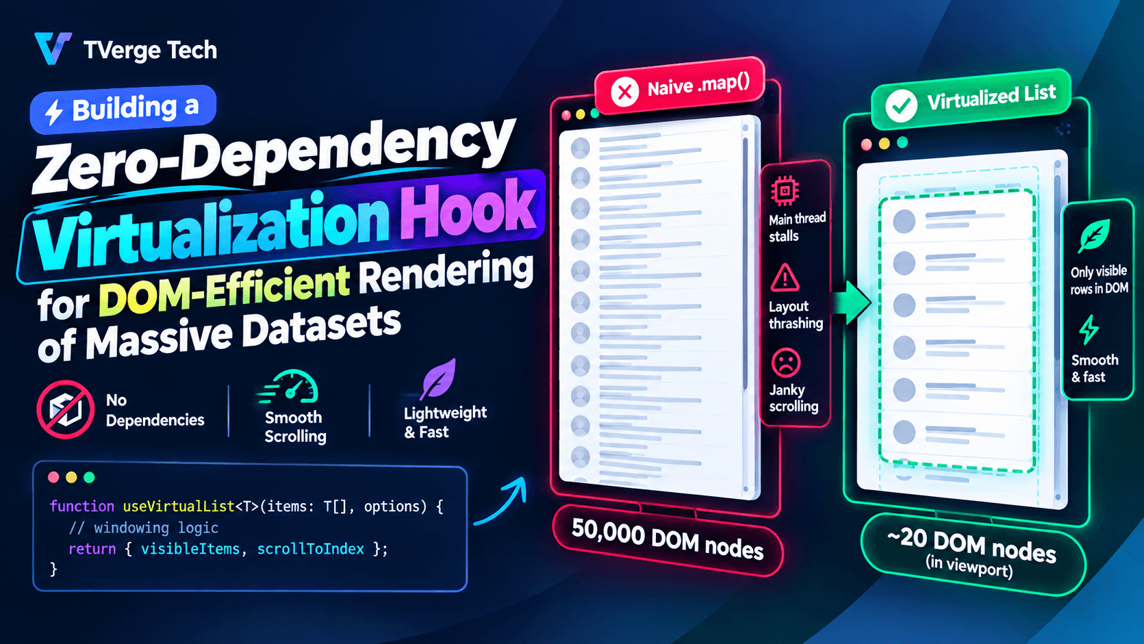
3Zero-Dependency Virtualization Hook: Render Massive Lists Fast